Using Linear Regression to Predict House Prices
Exploring multivariable regression to model and predict valuations using multiple data inputs. Demonstrating how statistical analysis and machine learning techniques can be applied to estimate real-world values with accuracy.
The Data
The data for this project consists of records describing a suburb or town in Boston, each record has values for:
- CRIM: Per capita crime rate per town
- ZN: Proportion of residential land zoned for lots over 25,000sq.ft.
- INDUS: Proportion of non-retail business acres per town
- CHAS: Charles River dummy variable (= 1 if tract bounds river; 0 otherwise)
- NOX: Nitric oxides concentration (parts per 10 million)
- RM: Average number of rooms per dwelling
- AGE: Proportion of owner-occupied units built prior to 1940
- DIS: Weighted distances to five Boston employment centers
- RAD: Index of accessibility to radial highways
- TAX: Full-value property-tax rate per $10,000
- PTRATIO: Pupil-teacher ratio by town
- B: 1000(Bk−0.63)^2 where Bk is the proportion of black people by town
- LSTAT: % lower status of the population
The data comes from the Boston Standard Metropolitan Statistical Area (SMSA) in 1970.
Preliminary Data Exploration
The first step of working with a data set such as this, is some basic data exploration and cleaning. Looking at the column names, as well as checking for NaN values and duplicates - removing such values where appropriate.
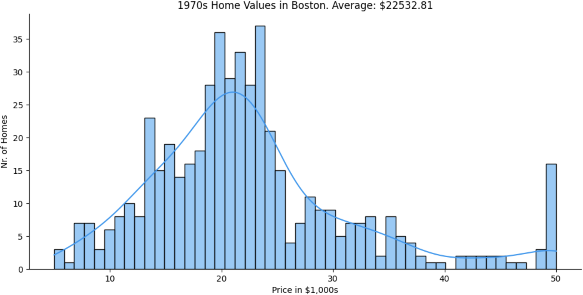
The following visualisations were created with Seaborn. You can see a Kernel Density Estimate (KDE) curve overlaid on each of the histograms.
Predicting House Prices
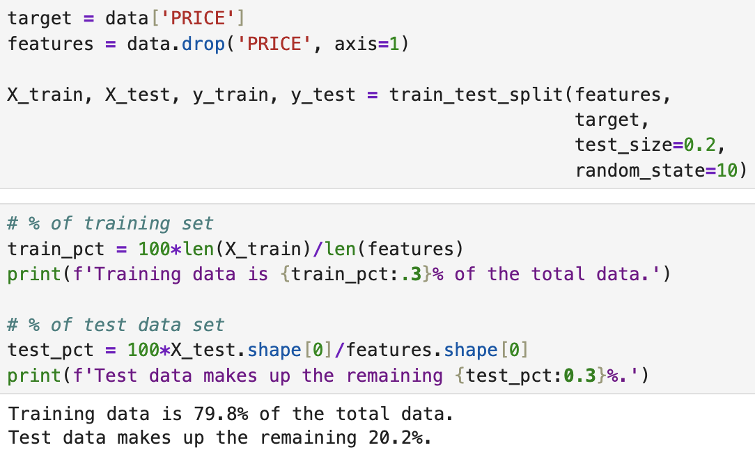
In order to train a model which can predict house prices for us, we need to split our data into testing and training sets, each with the 'features': those metrics by which we get the 'target' value. In this case the target value is the price, so the features will be all over values, i.e. CRIM, RM, TAX, etc.
I'm using sklearn for this part of the project, namely the test_train_split() function.
Multivariable Regression
PRICE = ϴ0 + ϴ1RM + ϴ2NOX + ϴ3DIS + ϴ4CHAS... + ϴ13LSTAT
Running the First Regression
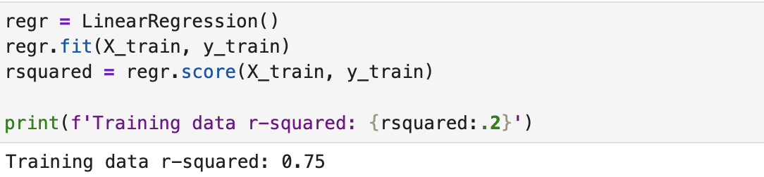
After running regression on the training dataset we get an R-squared value of 0.75. What does that actually mean? R-squared is the fraction by which the variance of the errors is less than the variance of the dependent variable.
Evaluating the Coefficients of the Model
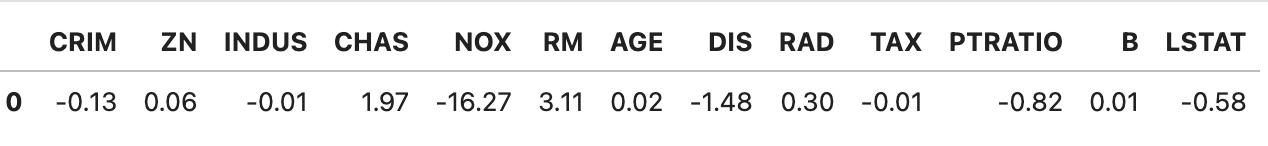
We can do a sanity check here, to see if the coefficients are what we might expect. Those coefficients with negative values would be indicative of an area with cheaper housing: higher crime-rate, more pollution in the air, a higher pupil-to-teacher ratio in schools. From looking, it appears that our coefficients are what we might expect at this point.
One thing we can see from these coefficients, and the equation we have above, is that an extra room in a house in 1970s Boston would add about $3,100 to the value of the house!
Residuals
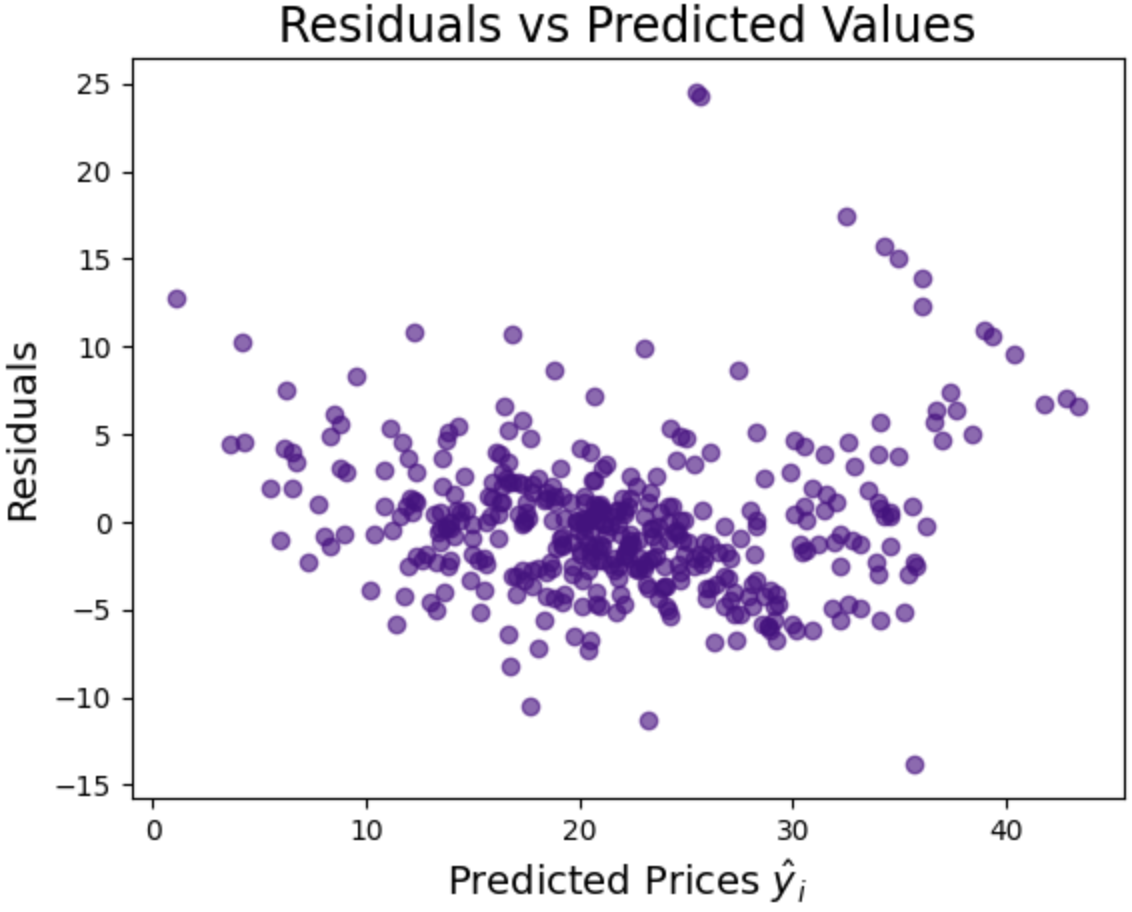
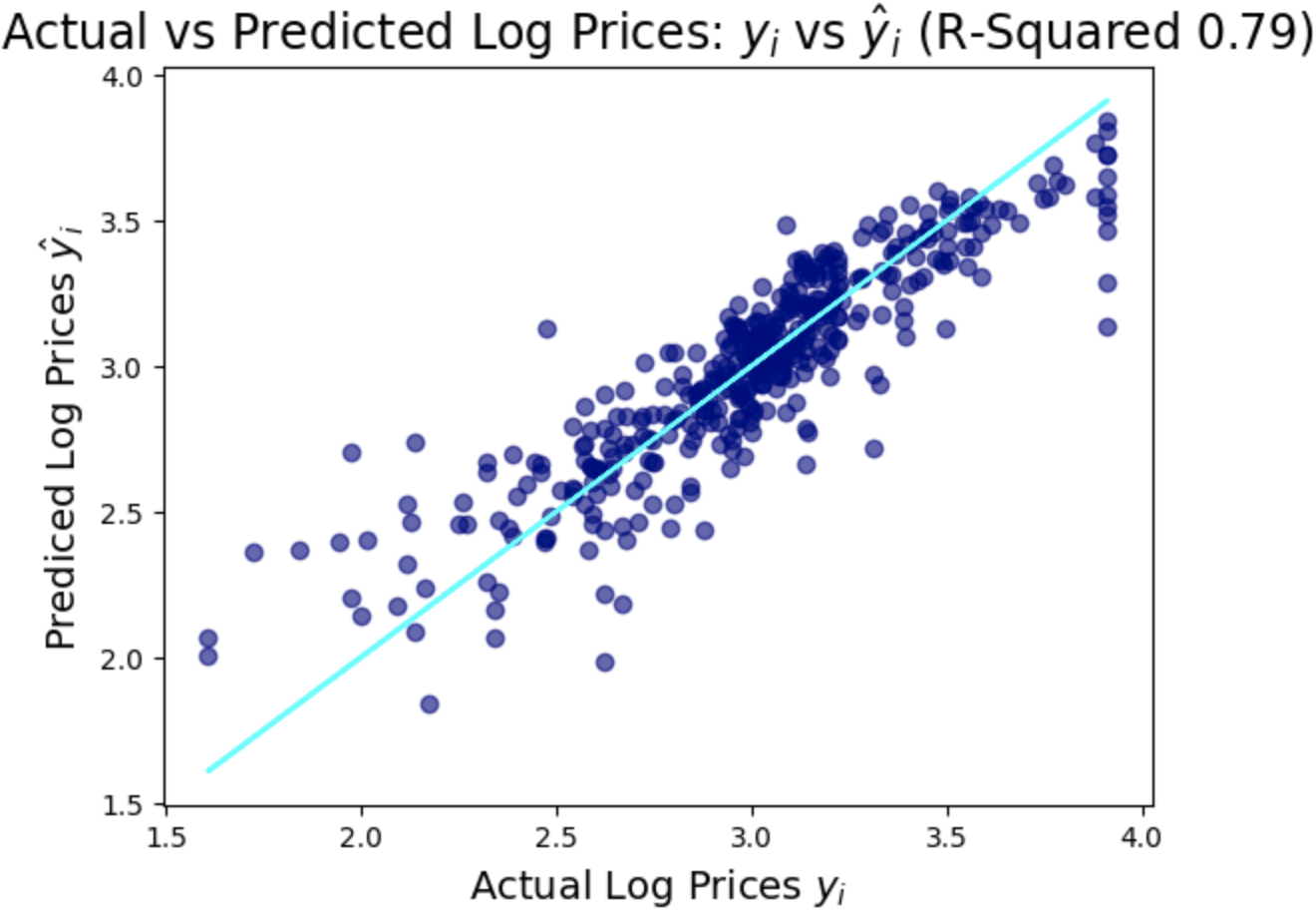
Another means by which we might evaluate our regression is residuals - the difference between the model's predictions (ŷi) and the true values (yi).
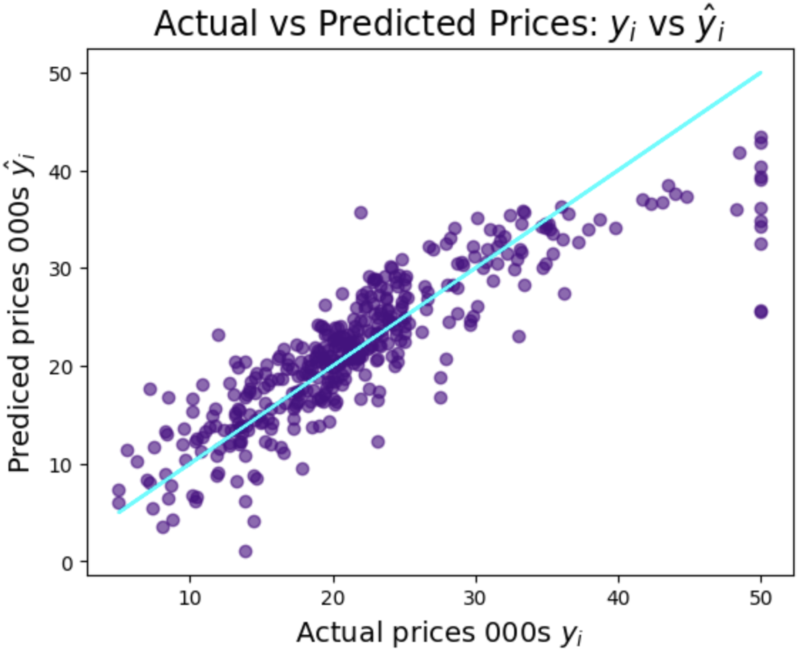
You can see on the first graph, of predicted vs actual prices (where predicted prices are represented by the light blue line) that the predictions are pretty good. Where the accuracy of the predictions seems to drop off is at the more expensive end of the scale. Perhaps we need to make some adjustments...
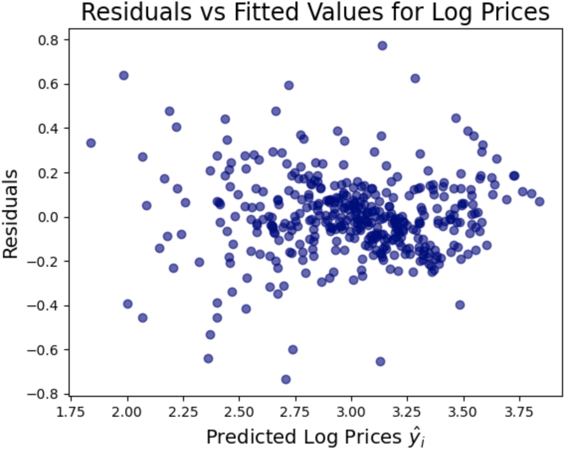
The second graph shows us the residuals from our model. It looks a bit random, but that's what we want. If our errors had a pattern, it would suggest systematic bias.
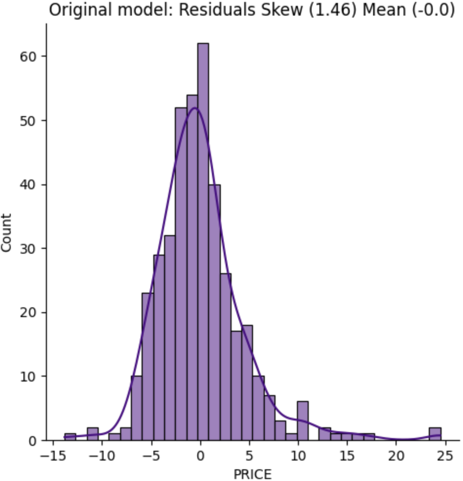
When looking at the skew of the residuals, we ideally want to see a normal distribution, a skewness and mean of 0. A skewness of 0 means the distribution is symmetrical, not biased in either direction. In our case we have a result of 1.46, and perhaps we could transform our data to get a better result.
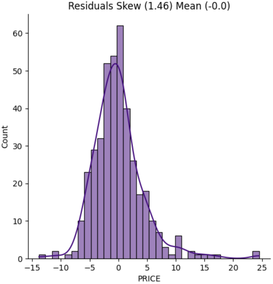
If we plot the log of the prices on a histogram, we get a skew of -0.33, or about a third of the skew for normal prices.
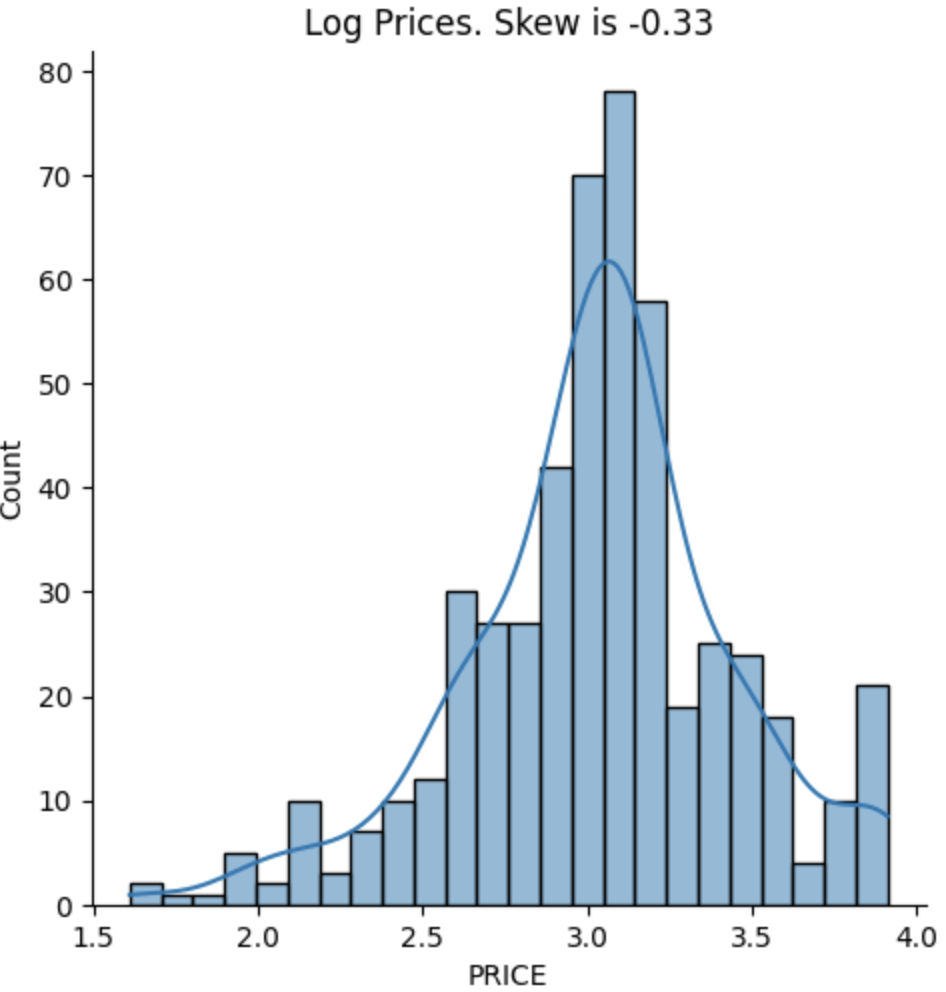
Let's try another regression, this time using the log of the prices.
log(PRICE) = ϴ0 + ϴ1RM + ϴ2NOX + ϴ3DIS + ϴ4CHAS... + ϴ13LSTAT
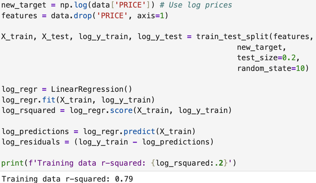
An R-squared value of 0.79 is a slight improvement over the earlier 0.75.
Evaluating the Coefficients of the Model (log)

The signs of the values are as before, those metrics which you might expect to reduce the value of a property have not changed.
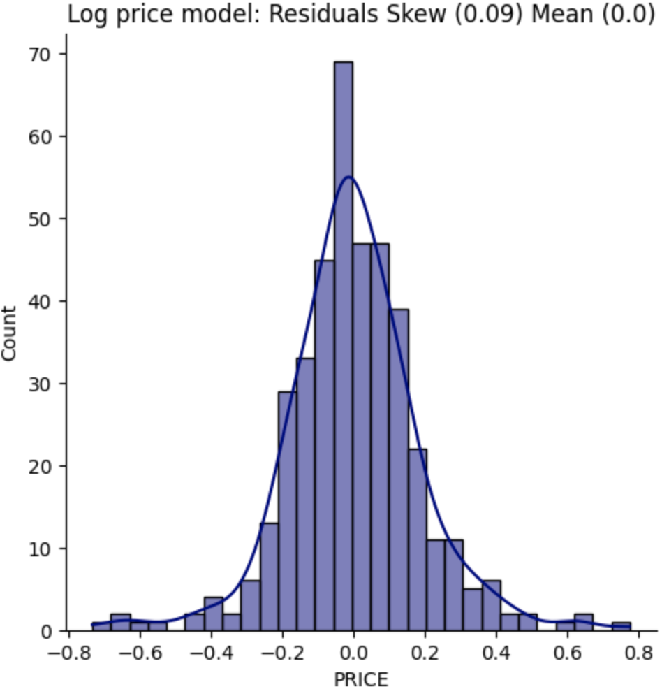
We've made a big improvement on the skew of our model, combined with the R-squared improvement, it seems using a logarithmic approach may give us a better model.
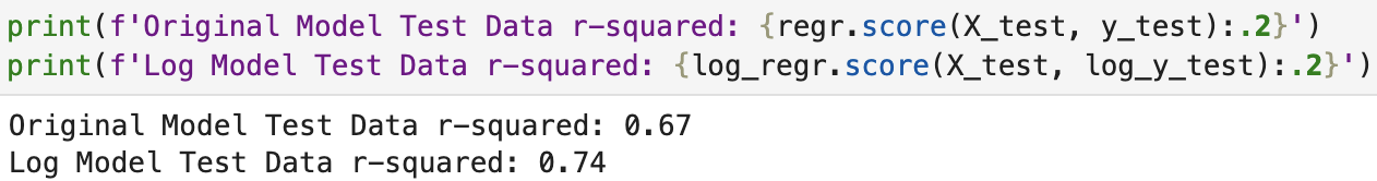
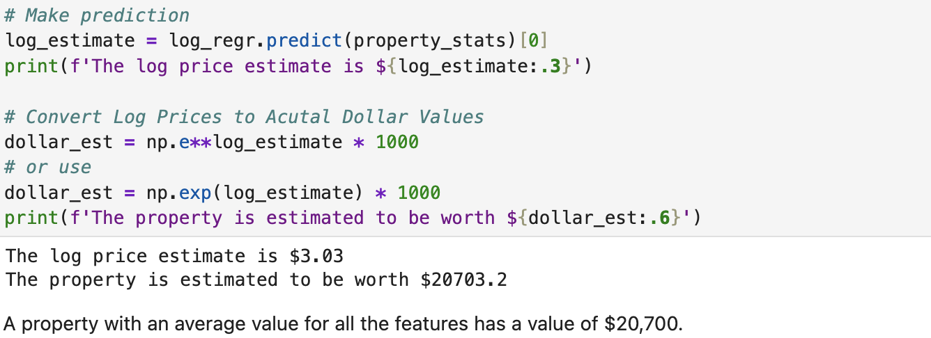
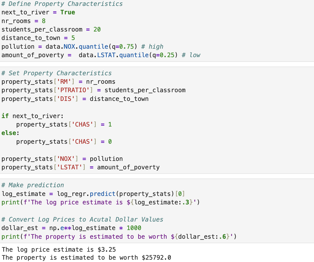
With our new model and coefficients, we can start to predict house prices for given metrics.
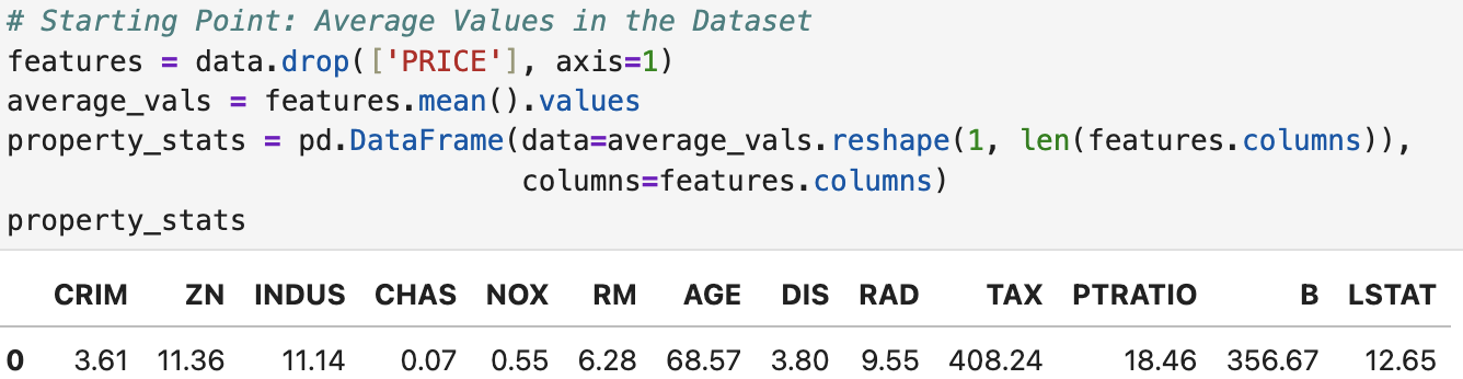
If we average all of the metrics we measure a property's value by in our dataset, we can make a prediction for the price of an average property.